Physics Lab

The Motion Sensor Demystified

(uses a Pasco Interface)

[Lab Index]

BHS -> Staff -> Mr. Stanbrough -> AP Physics-> Kinematics-> this page

Purpose:

To figure out how a motion sensor determines position, velocity, and acceleration.
To see how these calculations can be improved upon in some situations.

Discussion:

Undoubtedly, you have used a motion sensor and computer interface in other classes to plot graphs of position, velocity, and acceleration versus time, but how does the "magic box" do its "magic"? In physics, we don't want to treat laboratory equipment as "magic boxes" any more than we have to, and calculations of position, velocity, and acceleration are certainly something that we should be able to understand.

The motion sensor sends out a series of ultrasonic pulses. These pulses reflect from nearby objects and return to a detector. The computer software provides a very precise timer to measure the time elapsed between the sending of the original pulse and the detection of the reflected pulse.

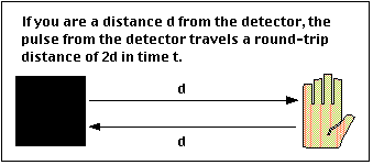detector distance graphic The pulses travel at the speed of sound in air, v (about 345 m/s, depending on atmospheric conditions). Suppose that the pulses reflect off an object that is a distance d from the motion sensor, and that the reflected pulse returns to the detector after time t. It's a simple application of "distance equals rate times time", except that the distance traveled by the pulse is 2d:

2d = vt, so
(Equation 1)

Your velocity is the slope (derivative) of your position vs. time graph, so if you were at position d₁ at time t₁, and position d₂ at time t₂, your velocity can be approximated as:

(Equation 2)

In the same way, your acceleration is the slope (derivative) of your velocity vs. time graph, so if you have velocity v₁ at time t₁, and velocity v₂ at time t₂, your acceleration will be approximately:

(Equation 3)

Equipment:

Pasco Science Workshop^TM interface

Motion Detector

air track & glider or dynamics track (optional)

Setting Up:

You can set up the motion detector to measure a motion that you create, or the motion of a glider on a sloping air track - whatever. The actual motion isn't the point here, just its analysis.

Setting Up the Pasco Interface:

Hint:

Turn on "Show Balloons" in the Help Menu. It will explain the purpose of the various icons in the Pasco interface - which is a big help.

Hook up and initialize the Pasco Science Workshop^TM interface.
Set up the motion sensor () to detect your motion.
1. You can either stop the sensor manually (), or go to the "Sampling Options" screen () and set a stop time appropriate for your motion.
Create a graph () to display position, velocity, and acceleration for your motion.
Resize and arrange the windows for a convenient display.

Procedure:

Record a motion or two - we just need some data to look at.

Analysis:

Position:

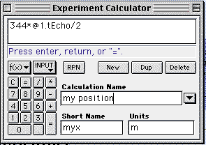
Compare this formula to equation 1 above. The default speed of sound (344 m/s - If you calibrated the motion sensor to some other value, use it here. Did you forget it? Double-click the motion sensor icon ()) was used in this calculation, and the "@1.tEcho" comes from the "Input" menu. It would be more efficient to use "172*@1.tEcho", but what I have looks more like equation 1.

How does the motion sensor know where you are? Not by magic - it uses equation 1 above! Here's how you can verify this claim:

Create a data table to display "Sonic Pulse Round Trip Time". Add a column for "Position".
To create your own position calculation using equation 1, open the Experiment Calculator, and enter the new calculation shown at right.
Add a column to your data table to display this calculation, and compare it to the motion sensor's position data. You could also add a graph of myx vs. time, and compare to the original. Neat, huh?

Velocity:

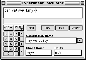
Here is the calculation for the velocity. The "derivative" comes from the f(x) - Special menu, and the myx comes from the "INPUT" menu. The "4" means that the program calculates the slope between the current time and 4 time intervals later.

Add a velocity column to your data table.

Go to the Experiment Calculator, and add the new calculation shown at right. Science Workshop^TM doesn't allow you (as far as I know) to enter a calculation like equation 2 directly, but the Derivative() function uses this method to calculate a numerical derivative.
Add a column to your data table to display the velocity calculation, and compare it to the motion sensor's calculation.

Acceleration:

acceleration calculation

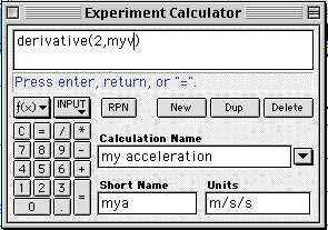
The calculation for acceleration is shown above. Why "2" here and "4" above? I don't know - but it matches the Science Workshop^TM calculation though, doesn't it?

The calculation that Science Workshop^TM uses for acceleration is similar (as it should be) to the one for velocity. To check it out:

Add an acceleration column to your data table.
Create a calculation for acceleration in the Experiment Calculator, and add it to the data table.

Possible Improvements:

Now that you know how the motion sensor determines your position, velocity, and acceleration, you can go ahead and use the built-in calculations when you need them, you don't have to create your own calculations each time. I'm sure that you've noticed that the kinematics graphs produced by the motion sensor are sometimes (ok, often - well, generally) pretty rough - especially the acceleration vs. time graphs. This is because slight irregularities in the round-trip times show up as irregularities in the position data, which are magnified in the velocity calculation, then magnified again in the acceleration calculation.

What can you do? First, you should make sure that the motion detector is not getting reflections from some unwanted object. Try clearing the area, re-aiming the detector, and adjusting the beam (near/far). This probably won't remove all of the "jitters" in the data, but it can help a lot. Beyond that, you can either work around it, or try to fix it.

Curve Fitting:

acceleration vs. time graph

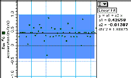
To create acceleration vs. time graph shown above:

Zoom in () on the region you want to examine.

Highlight the region in which you want the curve fit using the mouse.

Select a curve fit for the data.

To work around the problem and ignore the "noise" in the data, you could try a curve fit. For instance, suppose your acceleration vs. time graph looks linear, but really noisy. Try this:

Go to the graph options dialog (), and turn off "Connected Points". ("Connected Points" are usually a bad idea, anyway!)
Try a curve fit - remember that you can restrict the curve fit to a particular region of the data.

Smoothing the Data:

Smoothed x calculation window

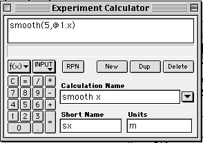
The Experiment Calculator window shown above displays a smoothing function applied to motion sensor position data. The "smooth" function is found in the "Special" submenu of the "f(x)" menu, and the "@1.x" is found in the "INPUT" menu.

"Smoothing" is a statistical process that tends to do just that - smooth out the "jumps and jiggles" in a data set. It does so by averaging the current value with a certain number of adjacent points.

Well, doesn't that change the data? Yes, it does. Isn't that somehow underhanded and unsavory, if not downright illegal? Well, no, it isn't. If the "jumps and jiggles" are truly random noise (just about the same number of high and low jumps, etc.), then there is nothing wrong with trying to remove it. Just be sure to:

keep the original data, and
properly label the smoothed data.

Science Workshop^TM makes it easy to smooth a data set. In the "Special" submenu of the "f(x)" menu in the Experiment Calculator window you will find the "smooth(n, x)" function. Here, "x" is the data set to smooth, and "n" is the number of points to use in the smoothing operation. How many points should you use? You need to play around with it. Too few, and the data isn't really affected by the smoothing operation, and too many can remove a great deal of the information content. It's a judgment call.

Smoothed acceleration graph

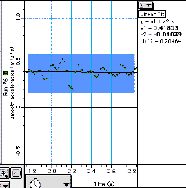
This graph uses the same data as the graph above, but the original round-trip time data (only) was moderately smoothed (n = 5).

Go ahead and apply the smoothing operation to your motion detector position data, as shown in the example at right. (You could, instead, smooth the original round-trip time data.) Add it to your data table and compare the smoothed values to the raw data. You might also want to compare their graphs. Try different numbers of points to see what happens. (Since the position data taken by the motion detector isn't particularly "noisy", you probably won't notice any radical differences.)

Now, modify your velocity calculation to use the smoothed position values instead of the raw data, and compare. You can smooth the new velocity data, too. Now modify your acceleration calculation to use the smoothed velocity data, etc. (That's a lot of smoothing - it is possible to "go nuts" with this smoothing thing, you know...) What do you think?

Conclusions:

Hopefully, this lab exercise has given you an understanding of how the motion detector does its detecting, as well as some steps to take to improve the process that you can apply in your future work.